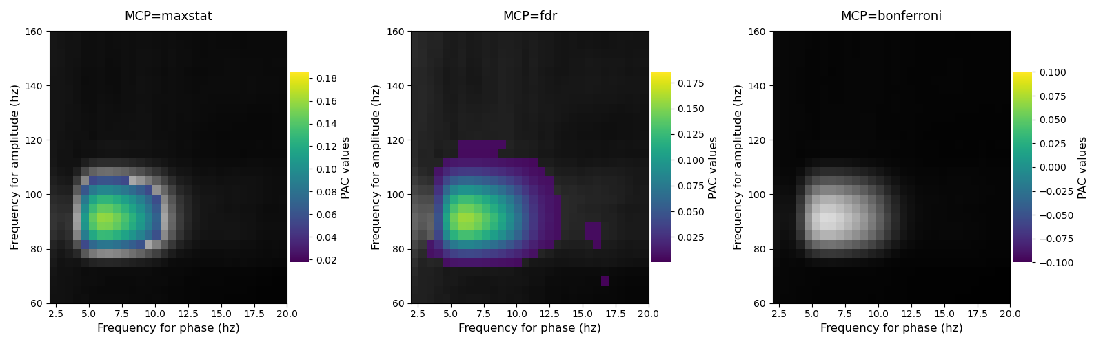
Comparison of methods for correcting p-values for multiple comparisons

This script illustrates three methods to correct the p-values for multiple comparisons (i.e by the number of phases and by the number of amplitudes) :

• Using the maximum statistics

• Using a FDR correction

• Using a Bonferroni correction

Note that for the FDR and Bonferroni corrections, MNE-Python is needed.

import numpy as np

from tensorpac import Pac
from tensorpac.signals import pac_signals_wavelet

import matplotlib.pyplot as plt

Simulate artificial coupling

first, we generate several trials that contains a coupling between a 6z phase and a 90hz amplitude. By default, the returned dataset is organized as (n_epochs, n_times) where n_times is the number of time points and n_epochs is the number of trials

f_pha = 6       # frequency phase for the coupling
f_amp = 90      # frequency amplitude for the coupling
n_epochs = 30   # number of trials
n_times = 4000  # number of time points
sf = 512.       # sampling frequency
data, time = pac_signals_wavelet(f_pha=f_pha, f_amp=f_amp, noise=.4,
                                 n_epochs=n_epochs, n_times=n_times, sf=sf)

Compute true PAC estimation and surrogates distribution

Now, we compute the PAC using multiple phases and amplitudes such as the distribution of surrogates. In this example, we used the method proposed by Tort et al. 2010 [11]. This method consists in swapping phase and amplitude trials. Then, we used the method tensorpac.Pac.infer_pvalues in order to get the corrected p-values across all possible (phase, amplitude) frequency pairs.

# define the Pac object
p = Pac(idpac=(1, 1, 0), f_pha='mres', f_amp='mres')
# compute true pac and surrogates
n_perm = 200  # number of permutations
xpac = p.filterfit(sf, data, n_perm=n_perm, n_jobs=-1).squeeze()

plt.figure(figsize=(16, 5))
for n_mcp, mcp in enumerate(['maxstat', 'fdr', 'bonferroni']):
    # get the corrected p-values
    pval = p.infer_pvalues(p=0.05, mcp=mcp)
    # set to gray non significant p-values and in color significant values
    pac_ns = xpac.copy()
    pac_ns[pval <= .05] = np.nan
    pac_s = xpac.copy()
    pac_s[pval > .05] = np.nan

    plt.subplot(1, 3, n_mcp + 1)
    p.comodulogram(pac_ns, cmap='gray', colorbar=False, vmin=np.nanmin(pac_ns),
                   vmax=np.nanmax(pac_ns))
    p.comodulogram(pac_s, title=f'MCP={mcp}', cmap='viridis',
                   vmin=np.nanmin(pac_s), vmax=np.nanmax(pac_s))
    plt.gca().invert_yaxis()

plt.tight_layout()
p.show()

Out:

/home/circleci/project/examples/stats/plot_compare_mcp.py:69: RuntimeWarning: All-NaN slice encountered
  vmin=np.nanmin(pac_s), vmax=np.nanmax(pac_s))