Compare PAC of two experimental conditions with cluster-based statistics

This example illustrates how to statistically compare the phase-amplitude coupling results coming from two experimental conditions. In particular, the script below a the cluster-based approach to correct for the multiple comparisons.

In order to work, this script requires MNE-Python package to be installed in order to perform the cluster-based correction (mne.stats.permutation_cluster_test())

import numpy as np

from tensorpac import Pac
from tensorpac.signals import pac_signals_wavelet

from mne.stats import permutation_cluster_test

import matplotlib.pyplot as plt

Simulate the data coming from two experimental conditions

Let’s start by simulating data coming from two experimental conditions. The first dataset is going to simulate a 10hz phase <-> 120hz amplitude coupling while the second dataset will not include any coupling (random data)

# create the first dataset with a 10hz <-> 100hz coupling
n_epochs = 30   # number of datasets
sf = 512.       # sampling frequency
n_times = 4000  # Number of time points
x_1, time = pac_signals_wavelet(sf=sf, f_pha=10, f_amp=120, noise=2.,
                             n_epochs=n_epochs, n_times=n_times)
# create a second random dataset without any coupling
x_2 = np.random.rand(n_epochs, n_times)

Compute the single trial PAC on both datasets

once the datasets created, we can now extract the PAC, computed across time-points for each trials and across several phase and amplitude frequencies

# create the pac object. Use the Gaussian-Copula PAC
p = Pac(idpac=(6, 0, 0), f_pha='hres', f_amp='hres', dcomplex='wavelet')
# compute pac for both dataset
pac_1 = p.filterfit(sf, x_1, n_jobs=-1)
pac_2 = p.filterfit(sf, x_2, n_jobs=-1)

Correct for multiple-comparisons using a cluster-based approach

Then, we perform the cluster-based correction for multiple comparisons between the PAC coming from the two conditions. To this end we use the Python package MNE-Python and in particular, the function mne.stats.permutation_cluster_test()

# mne requires that the first is represented by the number of trials (n_epochs)
# Therefore, we transpose the output PACs of both conditions
pac_r1 = np.transpose(pac_1, (2, 0, 1))
pac_r2 = np.transpose(pac_2, (2, 0, 1))

n_perm = 1000  # number of permutations
tail = 1       # only inspect the upper tail of the distribution
# perform the correction
t_obs, clusters, cluster_p_values, h0 = permutation_cluster_test(
    [pac_r1, pac_r2], n_permutations=n_perm, tail=tail)

Out:

Using a threshold of 4.006873
/home/circleci/project/examples/stats/plot_compare_cond_cluster.py:71: DeprecationWarning: The default for "out_type" will change from "mask" to "indices" in version 0.22. To avoid this warning, explicitly set "out_type" to one of its string values.
  [pac_r1, pac_r2], n_permutations=n_perm, tail=tail)
stat_fun(H1): min=0.000000 max=52.333180
Running initial clustering
Found 13 clusters
Permuting 999 times...

  0%|          |  : 0/999 [00:00<?,       ?it/s]
  3%|2         |  : 25/999 [00:00<00:01,  710.88it/s]
  5%|5         |  : 53/999 [00:00<00:01,  715.89it/s]
  8%|7         |  : 77/999 [00:00<00:01,  715.62it/s]
 11%|#         |  : 106/999 [00:00<00:01,  721.62it/s]
 14%|#3        |  : 135/999 [00:00<00:01,  727.40it/s]
 16%|#5        |  : 158/999 [00:00<00:01,  724.90it/s]
 19%|#8        |  : 187/999 [00:00<00:01,  730.49it/s]
 22%|##1       |  : 215/999 [00:00<00:01,  734.75it/s]
 24%|##4       |  : 241/999 [00:00<00:01,  736.31it/s]
 27%|##6       |  : 268/999 [00:00<00:00,  739.12it/s]
 29%|##9       |  : 291/999 [00:00<00:00,  735.92it/s]
 31%|###1      |  : 311/999 [00:00<00:00,  727.03it/s]
 33%|###3      |  : 330/999 [00:00<00:00,  716.55it/s]
 35%|###5      |  : 353/999 [00:00<00:00,  714.59it/s]
 38%|###8      |  : 380/999 [00:00<00:00,  718.31it/s]
 41%|####1     |  : 411/999 [00:00<00:00,  726.10it/s]
 44%|####3     |  : 435/999 [00:00<00:00,  725.21it/s]
 46%|####6     |  : 461/999 [00:00<00:00,  727.15it/s]
 49%|####9     |  : 493/999 [00:00<00:00,  735.62it/s]
 51%|#####1    |  : 512/999 [00:00<00:00,  724.28it/s]
 53%|#####3    |  : 530/999 [00:00<00:00,  711.37it/s]
 55%|#####4    |  : 549/999 [00:00<00:00,  702.08it/s]
 57%|#####6    |  : 566/999 [00:00<00:00,  688.17it/s]
 59%|#####8    |  : 587/999 [00:00<00:00,  684.39it/s]
 61%|######    |  : 608/999 [00:00<00:00,  680.84it/s]
 64%|######3   |  : 635/999 [00:00<00:00,  685.91it/s]
 66%|######5   |  : 659/999 [00:00<00:00,  686.73it/s]
 68%|######7   |  : 679/999 [00:00<00:00,  681.28it/s]
 70%|######9   |  : 699/999 [00:00<00:00,  676.08it/s]
 72%|#######2  |  : 720/999 [00:01<00:00,  673.11it/s]
 74%|#######4  |  : 743/999 [00:01<00:00,  673.24it/s]
 77%|#######6  |  : 769/999 [00:01<00:00,  677.48it/s]
 80%|#######9  |  : 795/999 [00:01<00:00,  681.57it/s]
 82%|########2 |  : 824/999 [00:01<00:00,  688.59it/s]
 85%|########5 |  : 852/999 [00:01<00:00,  694.45it/s]
 88%|########7 |  : 878/999 [00:01<00:00,  697.83it/s]
 91%|######### |  : 905/999 [00:01<00:00,  702.29it/s]
 94%|#########3|  : 937/999 [00:01<00:00,  711.50it/s]
 97%|#########6|  : 968/999 [00:01<00:00,  719.37it/s]
 99%|#########9|  : 994/999 [00:01<00:00,  721.72it/s]
100%|##########|  : 999/999 [00:01<00:00,  733.16it/s]
Computing cluster p-values
Done.

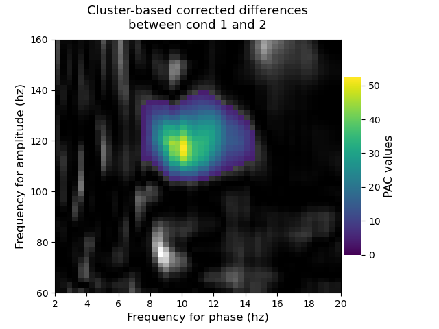
Plot the significant clusters

Finally, we plot the significant clusters. To this end, we used an elegant solution proposed by MNE where the non significant part appears using a gray scale colormap while significant clusters are going to be color coded.

# create new stats image with only significant clusters
t_obs_plot = np.nan * np.ones_like(t_obs)
for c, p_val in zip(clusters, cluster_p_values):
    if p_val <= 0.001:
        t_obs_plot[c] = t_obs[c]
        t_obs[c] = np.nan

title = 'Cluster-based corrected differences\nbetween cond 1 and 2'
p.comodulogram(t_obs, cmap='gray', colorbar=False)
p.comodulogram(t_obs_plot, cmap='viridis', title=title)
plt.gca().invert_yaxis()
plt.show()