Find the preferred phase (PP)

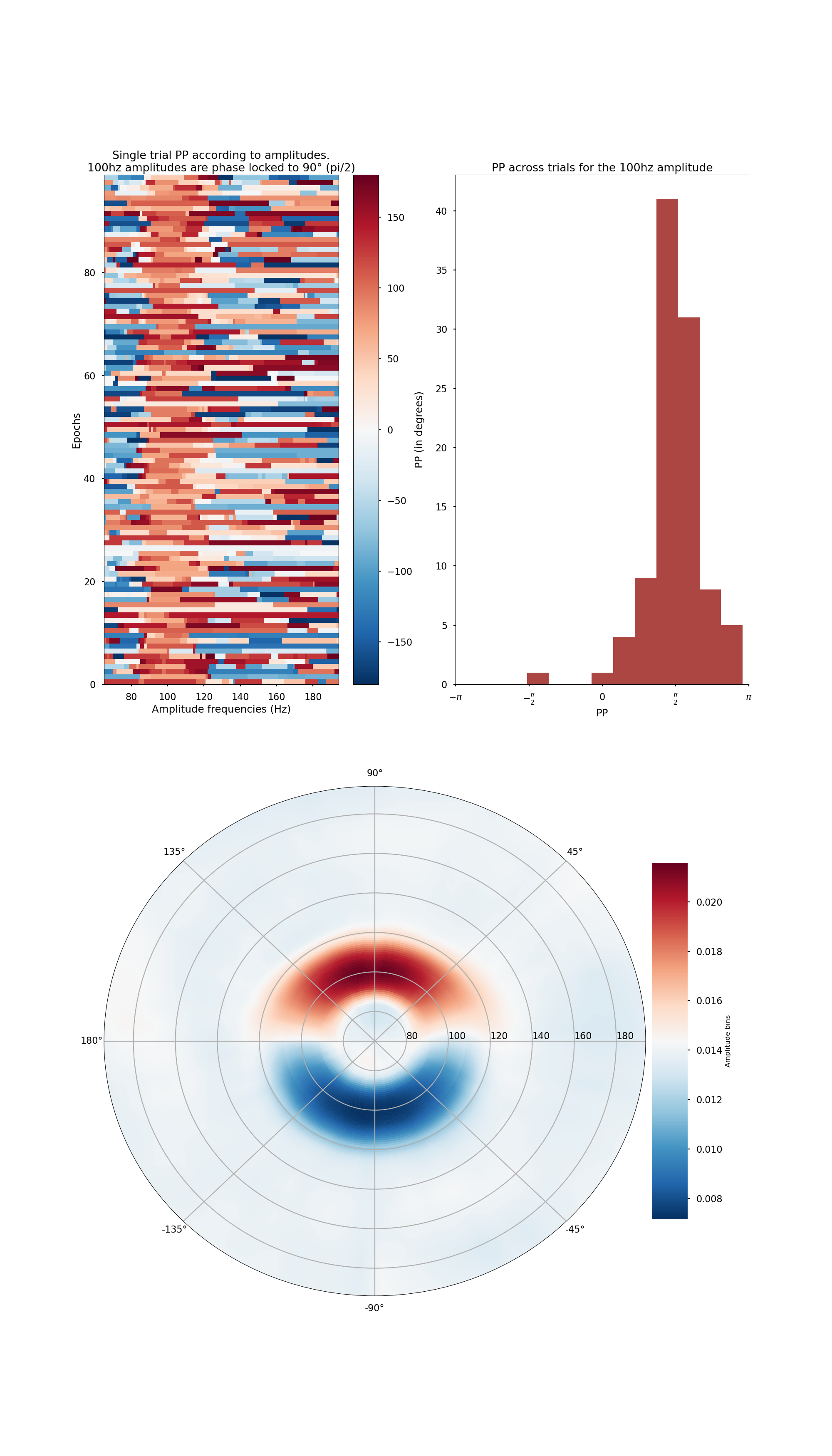
First, the amplitude is binned according to phase slices (360 degrees/nbins). Then, the PP is defined as the phase where the amplitude is maximum. We finally use the polar representation to display the preferred phase at different amplitudes.

import numpy as np

from tensorpac import PreferredPhase
from tensorpac.signals import pac_signals_wavelet

import matplotlib.pyplot as plt

plt.style.use('seaborn-poster')

Generate synthetic signals (sake of illustration)

to illustrate how does the preferred phase works, we generate synthetic signals where a 6hz phase is coupled with a 100hz amplitude. We also define a maximum amplitude at pi / 2

sf = 1024.
n_epochs = 100
n_times = 2000
pp = np.pi / 2
data, time = pac_signals_wavelet(f_pha=6, f_amp=100, n_epochs=n_epochs, sf=sf,
                                 noise=1, n_times=n_times, pp=pp)

Extract phases, amplitudes and compute the preferred phase

p = PreferredPhase(f_pha=[5, 7], f_amp=(60, 200, 10, 1))

# Extract the phase and the amplitude :
pha = p.filter(sf, data, ftype='phase', n_jobs=1)
amp = p.filter(sf, data, ftype='amplitude', n_jobs=1)

# Now, compute the PP :
ampbin, pp, vecbin = p.fit(pha, amp, n_bins=72)

Plot the preferred phase

Here, we first plot the preferred phase across trials according to amplitudes. Then, the distribution of 100hz amplitudes is first plotted according to the 72 phase bins and also using a polar representation

# Reshape the PP to be (n_epochs, n_amp) and the amplitude to be
# (nbins, n_amp, n_epochs). Finally, we take the mean across trials
pp = np.squeeze(pp).T
ampbin = np.squeeze(ampbin).mean(-1)

plt.figure(figsize=(20, 35))

# Plot the prefered phase
plt.subplot(221)
plt.pcolormesh(p.yvec, np.arange(100), np.rad2deg(pp), cmap='RdBu_r')
cb = plt.colorbar()
plt.clim(vmin=-180., vmax=180.)
plt.axis('tight')
plt.xlabel('Amplitude frequencies (Hz)')
plt.ylabel('Epochs')
plt.title("Single trial PP according to amplitudes.\n100hz amplitudes"
          " are phase locked to 90° (pi/2)")
cb.set_label('PP (in degrees)')

# Then, we show  the histogram corresponding to an 100hz amplitude :
idx100 = np.abs(p.yvec - 100.).argmin()
plt.subplot(222)
h = plt.hist(pp[:, idx100], color='#ab4642')
plt.xlim((-np.pi, np.pi))
plt.xlabel('PP')
plt.title('PP across trials for the 100hz amplitude')
plt.xticks([-np.pi, -np.pi / 2, 0, np.pi / 2, np.pi])
plt.gca().set_xticklabels([r"$-\pi$", r"$-\frac{\pi}{2}$", "$0$",
                          r"$\frac{\pi}{2}$", r"$\pi$"])

p.polar(ampbin.T, vecbin, p.yvec, cmap='RdBu_r', interp=.1, subplot=212,
        cblabel='Amplitude bins')

p.show()

Out:

/home/circleci/project/examples/misc/plot_preferred_phase.py:61: MatplotlibDeprecationWarning: shading='flat' when X and Y have the same dimensions as C is deprecated since 3.3.  Either specify the corners of the quadrilaterals with X and Y, or pass shading='auto', 'nearest' or 'gouraud', or set rcParams['pcolor.shading'].  This will become an error two minor releases later.
  plt.pcolormesh(p.yvec, np.arange(100), np.rad2deg(pp), cmap='RdBu_r')
/home/circleci/project/tensorpac/visu.py:133: MatplotlibDeprecationWarning: shading='flat' when X and Y have the same dimensions as C is deprecated since 3.3.  Either specify the corners of the quadrilaterals with X and Y, or pass shading='auto', 'nearest' or 'gouraud', or set rcParams['pcolor.shading'].  This will become an error two minor releases later.
  vmax=vmax, antialiased=True)