Comparison of the implemented PAC methods

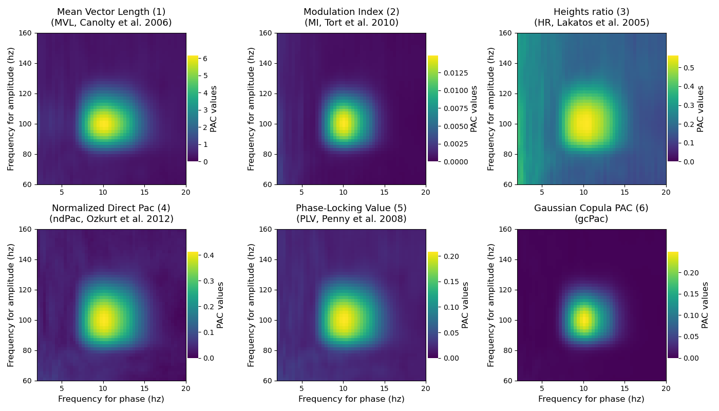
This script offers a comparison between all of the implemented PAC methods, in particular the methods that are computed across times-points.

from tensorpac import Pac
from tensorpac.signals import pac_signals_wavelet

import matplotlib.pyplot as plt

Simulate artificial coupling

first, we generate several trials that contains a coupling between a 10hz phase and a 100hz amplitude. By default, the returned dataset is organized as (n_epochs, n_times) where n_times is the number of time points and n_epochs is the number of trials

f_pha = 10      # frequency phase for the coupling
f_amp = 100     # frequency amplitude for the coupling
n_epochs = 20   # number of trials
n_times = 4000  # number of time points
sf = 512.       # sampling frequency
data, time = pac_signals_wavelet(sf=sf, f_pha=f_pha, f_amp=f_amp, noise=.8,
                              n_epochs=n_epochs, n_times=n_times)

Extract phases and amplitudes

Since we’re going to compute PAC using several methods, we’re first going to extract all of the phases and amplitudes only once

# define a pac object and extract high-resolution phases and amplitudes using
# Morlet's wavelets
p = Pac(f_pha='hres', f_amp='hres', dcomplex='wavelet')
# etract all of the phases and amplitudes
phases = p.filter(sf, data, ftype='phase', n_jobs=1)
amplitudes = p.filter(sf, data, ftype='amplitude', n_jobs=1)

Compute, plot and compare PAC

Once all of the phases and amplitudes extracted we can compute PAC by ietrating over the implemented methods.

plt.figure(figsize=(14, 8))
for i, k in enumerate([1, 2, 3, 4, 5, 6]):
    # switch method of PAC
    p.idpac = (k, 0, 0)
    # compute only the pac without filtering
    xpac = p.fit(phases, amplitudes)
    # plot
    plt.subplot(2, 3, k)
    title = p.method.replace(' (', f' ({k})\n(')
    p.comodulogram(xpac.mean(-1), title=title, cmap='viridis')
    if k <= 3:
        plt.xlabel('')

plt.tight_layout()
plt.show()