Compute and plot the Inter-Trial Coherence (ITC)

This example illustrate how to compute and plot the Inter-Trial Coherence (ITC). The ITC can be used to inspect if phases are aligned across trials or said differently, it provides a measure of the consistency across trials.

import numpy as np

from tensorpac.utils import ITC, PSD

import matplotlib.pyplot as plt

Generate a random data of shape (n_epochs, n_times)

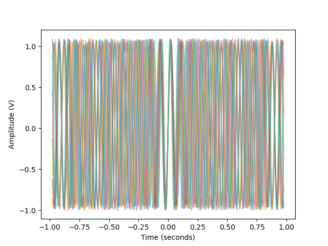
the dataset used in this example is composed of pure sines and noise. All sines across epochs are going to have a unique frequency so that there is no synchronization between them except around 0 second

# Let's start by creating a random dataset
n_epochs = 100  # number of trials
n_pts = 1000    # number of time points
sf = 512.       # sampling frequency
f_min = 10      # minimum sine frequency
f_max = 15      # maximum sine frequency

# create sines
time = np.linspace(-n_pts / 2, n_pts / 2, n_pts) / sf
freqs = np.linspace(f_min, f_max, n_epochs)
data = np.sin(2 * np.pi * freqs.reshape(-1, 1) * time.reshape(1, -1))
data += .1 * np.random.rand(n_epochs, n_pts)

# plot some trials and see how sines are synchronized around 0
trials = np.linspace(0, n_epochs - 1, 10).astype(int)
plt.figure(0)
plt.plot(time, data[trials, :].T, alpha=.5)
plt.xlabel('Time (seconds)'), plt.ylabel('Amplitude (V)')

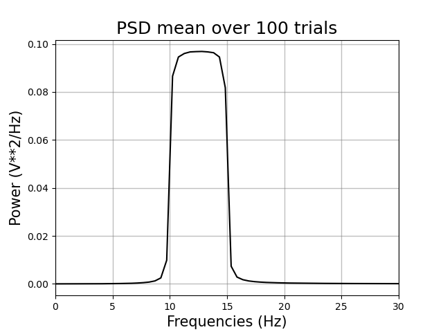
Compute and plot the Power Spectrum Density (PSD)

the PSD can also be used to inspect how frequencies are distributed across trials

psd = PSD(data, sf)
plt.figure(1)
psd.plot(f_max=30, confidence=None)

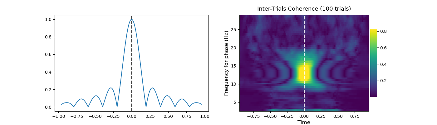
Compute and plot the Inter-Trial Coherence (ITC)

finally, compute and plot the ITC sphinx_gallery_thumbnail_number = 3

edges = 10  # remove 10 points to remove edge effects due to filtering
cycle = 6   # number of cycles to use to extract the phase

plt.figure(2, figsize=(14, 4))

# compute ITC for phases between [2, 30]Hz
itc = ITC(data, sf, f_pha=[f_min, f_max], edges=edges, cycle=cycle, n_jobs=1)
plt.subplot(121)
itc.plot(times=time)
plt.axvline(0, linestyle='--', color='black', lw=2)

# compute ITC for phases between [2, 30]Hz with frequency steps
itc = ITC(data, sf, f_pha=(2, 30, 1, .5), edges=edges, cycle=cycle, n_jobs=1)
plt.subplot(122)
itc.plot(times=time, cmap='viridis')
plt.axvline(0, linestyle='--', color='white', lw=2)
itc.show()