Generate artificially coupled signals

Use the pac_signals_tort function to generate artificial PAC.

from tensorpac.signals import pac_signals_tort
import matplotlib.pyplot as plt

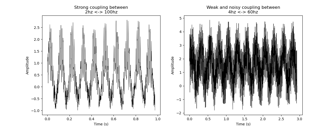
# Generate one signal containing PAC. By default, this signal present a
# coupling between a 2hz phase and a 100hz amplitude (2 <-> 100) :
sig, time = pac_signals_tort(n_epochs=1, n_times=1000)

# Now, we generate a longer and weaker 4 <-> 60 coupling using the chi
#  parameter. In addition, we increase the amount of noise :
sig2, time2 = pac_signals_tort(f_pha=4, f_amp=60, n_epochs=1, chi=.9,
                               noise=3, n_times=3000)

# Alternatively, you can generate multiple coupled signals :
sig3, time3 = pac_signals_tort(f_pha=10, f_amp=150, n_epochs=3, chi=0.5,
                               noise=2)

# Finally, if you want to add variability across generated signals, use the
# dpha and damp parameters :
sig4, time4 = pac_signals_tort(f_pha=10, f_amp=50, n_epochs=3, dpha=30,
                               damp=70, n_times=3000)


def plot(time, sig, title):
    """Plotting function."""
    plt.plot(time, sig.T, lw=.5, color='black')
    plt.title(title)
    plt.xlabel('Time (s)')
    plt.ylabel('Amplitude')


fig = plt.figure(figsize=(13, 5))
plt.subplot(1, 2, 1)
plot(time, sig, 'Strong coupling between\n2hz <-> 100hz')

plt.subplot(1, 2, 2)
plot(time2, sig2, 'Weak and noisy coupling between\n4hz <-> 60hz')

# plt.subplot(2, 2, 3)
# plot(time3, sig3, '3 signals coupled between 10hz <-> 150hz')

# plt.subplot(2, 2, 4)
# plot(time4, sig4, '3 signals coupled, with variability between 10hz <-> 50hz')

plt.show()