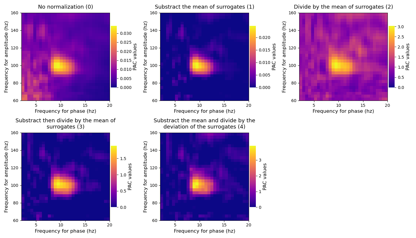
Compare normalization types

This example illustrates the effect of the different implemented normalizations. First, the true PAC is estimated, then this is the surrogate distribution that is estimated (i.e the PAC that could be obtained by chance). Finally, the true PAC is corrected by this distribution. Tensorpac includes four types of normalization that should give similar results :

• Substract the mean of surrogates (1)

• Divide by the mean of surrogates (2)

• Substract then divide by the mean of surrogates (3)

• Substract the mean then divide by the deviation of surrogates (z-score, 4)

from textwrap import wrap

from tensorpac import Pac
from tensorpac.signals import pac_signals_wavelet

import matplotlib.pyplot as plt

Simulate artificial coupling

first, we generate several trials that contains a coupling between a 10z phase and a 100hz amplitude. By default, the returned dataset is organized as (n_epochs, n_times) where n_times is the number of time points and n_epochs is the number of trials

f_pha = 10      # frequency phase for the coupling
f_amp = 100     # frequency amplitude for the coupling
n_epochs = 20   # number of trials
n_times = 2000  # number of time points
sf = 512.       # sampling frequency
data, time = pac_signals_wavelet(f_pha=f_pha, f_amp=f_amp, noise=2.,
                                 n_epochs=n_epochs, n_times=n_times, sf=sf)

Extract phases and amplitudes

now we can extract all of the phases and amplitudes

# define the pac object
p = Pac(f_pha='mres', f_amp='mres')
# Now, we want to compare PAC methods, hence it's useless to systematically
# filter the data. So we extract the phase and the amplitude only once
phases = p.filter(sf, data, ftype='phase', n_jobs=1)
amplitudes = p.filter(sf, data, ftype='amplitude', n_jobs=1)

Recompute PAC and surrogates and switch the normalization types

finally, we can recompute PAC and surrogates and then switch the normalization type. In particular this script uses the Gaussian-Copula PAC as the main measure and then permutes times blocks of amplitudes cut at a random time point

plt.figure(figsize=(14, 8))
for i, k in enumerate(range(5)):
    # switch the normalization method
    p.idpac = (6, 2, k)
    print('-> Normalization using ' + p.str_norm)
    # compute pac and surrogates (n_perm)
    xpac = p.fit(phases, amplitudes, n_perm=20)
    # plot
    plt.subplot(2, 3, k + 1)
    title = '\n'.join(wrap(f"{p.str_norm} ({k})", 40))
    p.comodulogram(xpac.mean(-1), title=title, cmap='plasma', vmin=0.)

plt.tight_layout()
plt.show()

Out:

-> Normalization using No normalization
-> Normalization using Substract the mean of surrogates
-> Normalization using Divide by the mean of surrogates
-> Normalization using Substract then divide by the mean of surrogates
-> Normalization using Substract the mean and divide by the deviation of the surrogates