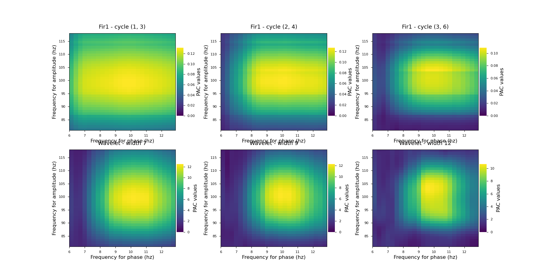
Compare filtering properties

Tensorpac provides two ways for extracting phase and amplitude :

• Using filtering followed by Hilbert transform.

• Using wavelets.

Out:

Filtering with fir1 filter
Filtering with wavelets

from __future__ import print_function
import matplotlib.pyplot as plt
from tensorpac import Pac
from tensorpac.signals import pac_signals_wavelet
plt.style.use('seaborn-paper')

# First, we generate a dataset of signals artificially coupled between 10hz
# and 100hz. By default, this dataset is organized as (ntrials, n_times) where
# n_times is the number of time points.
n_epochs = 5         # number of datasets
n_times = 4000  # number of time points
data, time = pac_signals_wavelet(f_pha=10, f_amp=100, noise=1.,
                                 n_epochs=n_epochs, n_times=n_times)

# First, let's use the MVL, without any further correction by surrogates :
p = Pac(idpac=(1, 0, 0), f_pha=(5, 14, 2, .3), f_amp=(80, 120, 2, 1),
        verbose=False)

plt.figure(figsize=(18, 9))
# Define several cycle options for the fir1 (eegfilt like) filter :
print('Filtering with fir1 filter')
for i, k in enumerate([(1, 3), (2, 4), (3, 6)]):
    p.cycle = k
    xpac = p.filterfit(1024, data, n_jobs=1)
    plt.subplot(2, 3, i + 1)
    p.comodulogram(xpac.mean(-1), title='Fir1 - cycle ' + str(k))

# Define several wavelet width :
p.dcomplex = 'wavelet'
print('Filtering with wavelets')
for i, k in enumerate([7, 9, 12]):
    p.width = k
    xpac = p.filterfit(1024, data)
    plt.subplot(2, 3, i + 4)
    p.comodulogram(xpac.mean(-1), title='Wavelet - width ' + str(k))

plt.show()