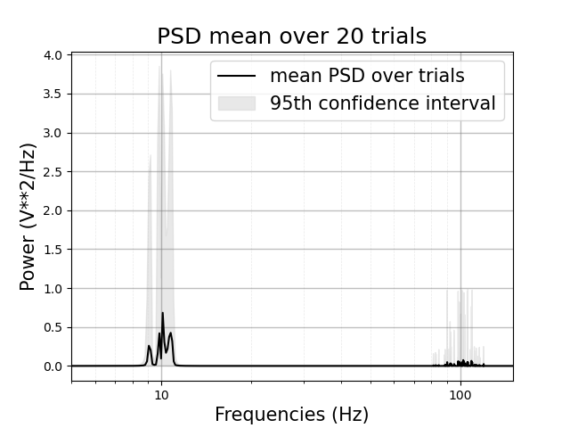
Compute and plot the Power Spectrum Density (PSD)

This example illustrate how to compute and plot the Power Spectrum Density (PSD) of an electrophysiological dataset. The PSD should be used to check that there is the presence of a clear peak, espacially for frequency phase.

Out:

/home/circleci/project/tensorpac/utils.py:208: MatplotlibDeprecationWarning: The 'basex' parameter of __init__() has been renamed 'base' since Matplotlib 3.3; support for the old name will be dropped two minor releases later.
  plt.xscale('log', basex=10)

from tensorpac.utils import PSD
from tensorpac.signals import pac_signals_tort

# Dataset of signals artificially coupled between 10hz and 100hz :
n_epochs = 20
n_times = 4000
sf = 512.  # sampling frequency

# Create artificially coupled signals using Tort method :
data, time = pac_signals_tort(f_pha=10, f_amp=100, noise=4, n_epochs=n_epochs,
                              dpha=10, damp=10, sf=sf, n_times=n_times)

# compute the PSD
psd = PSD(data, sf)

# plot the mean PSD across trials between [5, 150]Hz with a 95th confidence
# interval. Also, use a log x-scale
ax = psd.plot(confidence=95, f_min=5, f_max=150, log=True, grid=True)

# finally display the figure
psd.show()