Identify stationary time-series using unit root test

This example illustrates how to identify stationary time-series (i.e. time-series with constant statistical properties such as mean, variance etc.). Here, we are going to use the Augmented Dickey-Fuller test.

import numpy as np

from tensorpac.stats import test_stationarity

import matplotlib.pyplot as plt

Define a random dataset

Let first create a random dataset and change temporal properties

n_epochs = 8   # number of epochs
n_times = 200  # number of time points
sf = 128.

# create a reproducable random dataset
rng = np.random.RandomState(1)
data = rng.rand(n_epochs, n_times)
time = np.arange(n_times) / sf

# if we run the test on this random dataset, every epochs are going to be found
# as stationary as statistical properties are constant across time. Hence, we
# can introduce some randomness into this dataset to illustrate the sensibility
# of the test

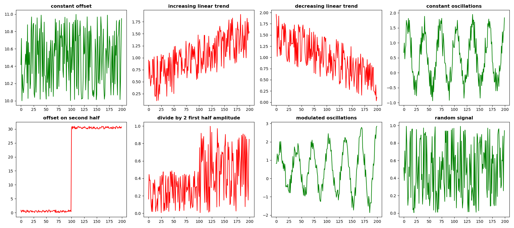
titles = {0: "constant offset", 1: "increasing linear trend",
          2: "decreasing linear trend", 3: "constant oscillations",
          4: "offset on second half", 5: "divide by 2 first half amplitude",
          6: "modulated oscillations", 7: "random signal"}

# Epoch 0 : constant offset
data[0, :] += 10.
data[1, :] += np.linspace(0, 1, n_times)
data[2, :] += np.linspace(1, 0, n_times)
data[3, :] += np.sin(2 * np.pi * 4 * time)
data[4, 100:] += 30.
data[5, 0:100] /= 2
data[6, :] += np.sin(2 * np.pi * 4 * time) * np.linspace(1, 2, n_times)

Compute the statistical test

now, run the Augmented Dickey-Fuller test in order to identify which trials are statisticaly considered as stationary

df = test_stationarity(data, p=0.05)
print(df)

Out:

    Epochs  ...   CV (1%)
0  epoch 0  ... -3.463815
1  epoch 1  ... -3.465244
2  epoch 2  ... -3.466005
3  epoch 3  ... -3.466398
4  epoch 4  ... -3.463645
5  epoch 5  ... -3.465059
6  epoch 6  ... -3.466398
7  epoch 7  ... -3.463645

[8 rows x 6 columns]

Plot each trial

finally, plot color-coded time-series (green : stationary, red: non-stationary)

colors = {True: 'green', False: 'red'}

is_stationary = df["Stationary"]

plt.figure(figsize=(18, 8))
for k in range(n_epochs):
    plt.subplot(2, 4, k + 1)
    plt.plot(data[k, :], color=colors[is_stationary[k]])
    plt.title(titles[k], fontweight='bold')
plt.tight_layout()
plt.show()